
How to Calculate Available Fire Flow from Hydrant Test Data: Formulas, Graphs & Worked Examples (NFPA 291)

When a hydrant test sheet lands on your desk—static, residual, pitot readings, outlet sizes—the number everyone needs is not the raw discharge. It is the available fire flow (AFF): how much water the system can still deliver when residual pressure is held at 20 psi. That single figure drives sprinkler demand checks, ISO grading, and whether a site plan survives design review.
NFPA 291 gives the field method and the math, but one path alone is easy to misapply. Wrong discharge coefficient, a single residual point stretched too far, or mixing AFF with rated capacity and needed fire flow (NFF) will put an indefensible number in the report. This article walks the three calculation routes side by side: the orifice/pitot formula, residual-pressure curve (or equation) projection to 20 psi, and rated-capacity classification. Worked examples with real static/residual/pitot data, multi-outlet cases, graphing versus calculation, and the setup mistakes that break accuracy show how to make the paths agree—and how to defend the result when they do not.
Why One Hydrant Test Sheet Can Yield Three Different Fire-Flow Numbers
They disagree. The same static, residual, and pitot readings can produce three legitimate but non-identical figures—available fire flow, rated capacity, and needed fire flow—because each answers a different question. Treat them as interchangeable and design or ISO numbers drift without anyone noticing.
Available fire flow (AFF) is the supply-side quantity the water system can deliver while residual pressure at the test hydrant stays at 20 psi. It is projected from the measured static pressure, residual pressure during flow, and pitot (or orifice) readings exactly as NFPA 291 practice requires. AFF is therefore a calculated system capacity at a fixed residual benchmark, not a raw outlet reading.
Rated capacity is simpler and more local. It states the flow the hydrant itself can discharge for a chosen pressure drop—commonly 10 psi or 20 psi below static—and is used for hydrant marking, color coding, and quick field labels. Because the drop is measured from static rather than locked to a 20 psi residual floor, rated capacity and AFF coincide only when static happens to sit near 40 psi; otherwise they diverge.
Needed fire flow (NFF) sits on the demand side. It is the target flow fire-protection engineers and ISO evaluators set for a building or occupancy. NFF consumes AFF results when adequacy is checked, yet it is never computed from pitot math; it comes from occupancy, construction, and exposure rules.
Utilities therefore quote rated capacity for asset records, sprinkler designers quote AFF at 20 psi for hydraulic calculations, and ISO quotes the relationship of AFF to NFF for public-protection scoring. One test sheet, three audiences. Running the orifice formula, the residual-pressure curve projection, and the rated-capacity classification side by side is what keeps those numbers from silently mismatching.
Lock Coefficients, Diameters, and Pressures Before You Run Any Formula
Those three routes only agree when every calculation starts from the same locked-in inputs. Before you touch a 20 psi projection, a rated-capacity drop, or the orifice math itself, fix coefficient C, outlet diameter, and the pressure readings that feed them. Get those wrong and all three methods drift together.
Choose C for the outlet you actually opened
The core pitot formula is Q = 29.83 × C × d² × √p, with Q in gpm when d is in inches and p is pitot pressure in psi. C is not a universal constant—it depends on how the outlet is finished. A smooth, well-rounded nozzle takes a higher coefficient than a square, sharp-edged opening or a tube that projects into the hydrant barrel. Worn seats, chipped lips, and damaged nozzles drift downward from the textbook value, so discharge shifts before any residual-pressure curve is drawn.
| Outlet condition | Typical C |
|---|---|
| Smooth and well-rounded | 0.90 |
| Square and sharp | 0.80 |
| Projecting into barrel / internal tube | 0.70 |
| Worn or damaged (field judgment) | Lower than nominal |
Lock diameter next. Measure the actual inside diameter of the outlet or nozzle tip in use—not the nominal hydrant size—and keep d and p in consistent units. Convert pitot psi to flow only after both diameter and C are fixed; swapping units mid-stream is a common source of silent error.
Match flowing outlets to the residual you recorded
When more than one outlet is open, compute each orifice flow with its own C, d, and pitot reading, then sum them for total test flow. The residual pressure on the sheet must belong to that same flowing set—mixing a single-outlet residual with a multi-outlet sum invalidates the two-point curve that Methods 1–3 will later share.
Elevation between the residual gauge and the flowing hydrant, or a gauge mounted well above the outlet centerline, also warps the static-to-residual drop. Note gauge height and ground-elevation differences on the sheet; ignoring them makes a clean NFPA 291 projection look cleaner than the hydraulics allow.
Pre-calc checklist (identical inputs for every method)
- Record static pressure at the residual hydrant with no flow.
- Identify every flowing outlet; measure actual inside diameter for each.
- Assign C from outlet finish (and condition), not from habit.
- Take pitot pressure at each flowing outlet; keep units inches and psi.
- Sum individual orifice flows only after C, d, and p are fixed per outlet.
- Confirm residual pressure was read against that exact flowing set.
- Note gauge height and any elevation difference between residual and flow hydrants.
- Only then hand the same static, residual, and total Q to Methods 1–3.
Method 1: From Test Flow to Available Fire Flow at 20 psi
Method 1 takes those three locked numbers—static pressure, residual pressure while flowing, and total pitot discharge Q—and projects the observed flow straight to the 20 psi residual that defines available fire flow.
Confirming Q from the orifice relation
Begin by verifying the test flow itself from the locked checklist values. Apply the orifice relation with the C, diameter, and pitot pressure already fixed for each nozzle, then sum every open outlet so the total is the QF you will scale. No further conversion is required once those inputs are set—the same total feeds the 20 psi projection below and the curve and rated-capacity paths that follow.
The NFPA 291 extrapolation
With QF confirmed, NFPA 291 supplies the single-step projection to 20 psi residual:
Q20 = QF × [(S − 20) / (S − R)]0.54
S is the static pressure recorded before any flow, R is the residual observed while discharging QF, and the exponent 0.54 approximates the pressure–flow relationship that appears on a typical municipal distribution system. The formula treats the drop from static to residual as friction-dominated loss in the mains rather than loss inside one hydrant barrel. On a strong, well-looped grid the projection is ordinarily trustworthy. On a weak or dead-end main the same exponent can over-predict available flow if the test already drove the system near its limit, or under-predict if local hydrant restrictions made the residual look lower than the true main pressure.
Which residual you may trust
That last point turns only on context, not on field technique. In a main-capacity test the residual gauge sits on a hydrant remote from the flowing outlets, so it reflects system pressure; in a hydrant-capacity test the residual is often taken on the flowing hydrant itself and therefore includes barrel and outlet losses. Feed the remote residual when the goal is system available fire flow; use the local residual only when you are characterizing that single hydrant. Either way, insert the chosen residual, the matching total Q, and static into the same 0.54 equation. The result is Method 1’s available fire flow at 20 psi—ready to be cross-checked against the residual-pressure curve and rated-capacity routes that follow.
Method 2: Building the Residual-Pressure Curve and Reading AFF at 20 psi
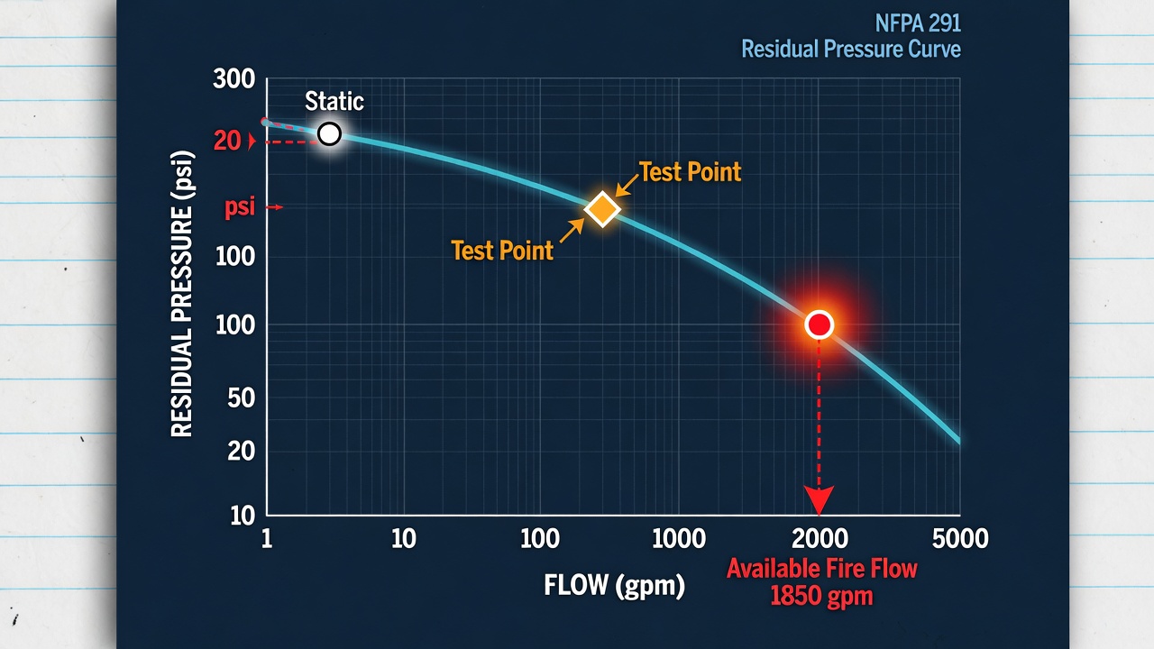
That Method 1 figure is only as trustworthy as a single-point extrapolation allows. Method 2 reconstructs the residual-pressure curve itself so you can read available fire flow directly at the 20 psi intercept—and see whether the formula and the graph agree—without returning to the field.
Plotting static and flowing points into a curve
Place residual pressure on the vertical axis (psi) and flow on the horizontal (gpm). Static pressure sits at zero flow. Each flowing test point—total pitot Q already locked against the residual measured while those outlets were open—becomes another coordinate on the same sheet. Draw a smooth curve through the points that follows the characteristic shape of friction head loss versus discharge (the same family of curves that underlies the 0.54 exponent). Two points define a usable curve; three or more reveal whether the system is behaving consistently and let you fair the line with far less guesswork between and beyond the measured rates.
Reading the 20 psi intercept and labeling for audit
Drop a horizontal line at 20 psi residual and read the flow where it crosses the curve. That intercept is Method 2’s available fire flow. Label both axes with units, mark the static point, every flowing test point with its Q and residual, the 20 psi line, and the intercept value itself. Anyone reviewing the sheet should be able to rebuild the graph and land on the same number.
When graph and formula should match—and when they should not
A few percent difference between the graphical intercept and Method 1’s Q20 result is normal: hand-drawn or spreadsheet curves smooth minor gauge scatter, and the exponent is itself an engineering approximation. Larger spreads almost always trace back to a mis-transcribed residual, an incorrect C or diameter in the pitot step, or an elevation/gauge-height error that shifted one of the locked inputs. Re-run the pre-calc checklist before trusting either figure. Sparse two-point tests still produce a defensible intercept, but the shape beyond the flowing point is assumed; each extra multi-outlet rate tightens the curve and makes the 20 psi reading far less sensitive to any single bad residual. When Method 1 and Method 2 land close, the available fire flow is ready for the rated-capacity cross-check that follows.
Method 3: Rated Capacity at a Fixed Pressure Drop—and When It Is Not AFF
That cross-check is Method 3. Rated capacity is calculated from the same locked pitot total Q, static, and residual, but it answers a different question: how much flow the hydrant (or the main at that hydrant) would deliver at a fixed pressure drop from static—commonly 10 psi or 20 psi—rather than at an absolute residual of 20 psi. Utilities use the figure for hydrant class labels and color codes; it is not automatically available fire flow.
The arithmetic reuses the familiar exponent. With test flow QF measured at observed drop (S − R), rated capacity at the chosen drop ΔPrated is simply Qrated = QF × (ΔPrated / (S − R))0.54. Same orifice-derived QF, same friction assumption, different target drop. Because the target is a relative drop instead of the 20 psi floor, the number can sit above or below the Method 1 / Method 2 AFF depending on static pressure and main strength. On a strong main with high static, the drop from static down to 20 psi residual is large, so Q20 exceeds the rated-capacity value computed for a modest fixed drop. On a weaker main whose static already sits near 40–50 psi, the absolute 20 psi residual is reached after only a small drop; the fixed-drop rated figure can then exceed true AFF and look deceptively generous.
That gap is exactly why a color-coded cap or a “rated 1,500 gpm” stencil must never be substituted for design available fire flow. The label encodes the utility’s chosen drop and class band; it does not prove residual pressure will still be 20 psi (or any other design residual) when that flow is taken. Print both numbers on the test summary—static, residual, total pitot Q, the Method 1 / Method 2 AFF at 20 psi, and, separately, rated capacity at the utility’s stated drop—so the residual basis stays visible. A sprinkler hydraulic model or ISO supply evaluation should pull the 20 psi AFF (or the residual-pressure curve itself). Rated capacity stays on the operations and labeling side of the handoff.
Full Worked Example: One Dataset Through All Three Methods
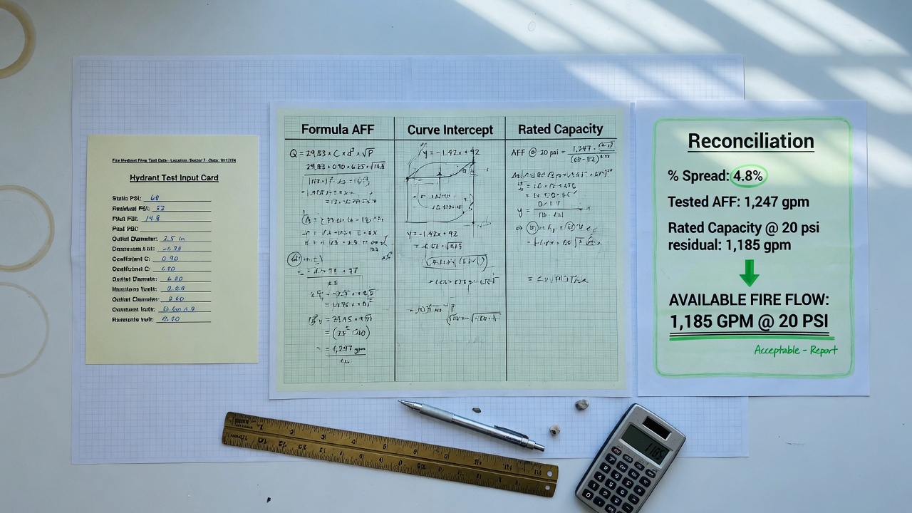
That handoff stays clean only when the same locked static, residual, and pitot totals are pushed through all three paths and the spread is written down side by side. The numbers below are ordinary field values; every root and power is shown so the arithmetic can be repeated by hand or in a spreadsheet.
Raw test sheet and pitot totals
Static pressure S = 68 psi. Two 2½-inch outlets, both smooth/rounded so C = 0.90, are opened together. Measured diameters are the true 2.50 in (d² = 6.25). Pitot on the first outlet reads 25.0 psi (√p = 5.000); pitot on the second reads 16.0 psi (√p = 4.000). Residual while both flow is R = 46 psi.
Orifice constant check: 29.83 × 0.90 = 26.847; 26.847 × 6.25 = 167.79. Then Q₁ = 167.79 × 5.000 = 838.95 gpm and Q₂ = 167.79 × 4.000 = 671.16 gpm. Summed test flow QF = 1,510 gpm. (Units stay gpm, inches, psi throughout; no conversion factors are required.)
Method 1 — formula AFF at 20 psi
Q20 = QF × [(S − 20)/(S − R)]0.54 = 1,510 × [(68 − 20)/(68 − 46)]0.54 = 1,510 × (48/22)0.54 = 1,510 × (2.1818)0.54. Square root of 2.1818 is 1.477; the remaining 0.04 power multiplies by approximately 1.032, giving 1.524. Therefore Q20 = 1,510 × 1.524 = 2,301 gpm.
Method 2 — residual-pressure curve intercept
Plot the zero-flow point (0 gpm, 68 psi) and the two-outlet point (1,510 gpm, 46 psi). Under the same 0.54 exponent the 20 psi intercept is identical to Method 1: 2,301 gpm. A single-outlet check point was also recorded—only the first butt open, pitot 36 psi (√p = 6), Q = 167.79 × 6 = 1,007 gpm, residual 55 psi. That third point lies on the same smooth curve, confirming the intercept is stable and that outlet aggregation has been handled correctly.
Method 3 — rated capacity at a 20 psi drop
For a rated drop of 20 psi from static, Qrated = QF × (20 / (S − R))0.54 = 1,510 × (20/22)0.54 = 1,510 × (0.9091)0.54. Square root 0.9535 times the small residual factor ≈ 0.950 yields Qrated = 1,435 gpm.
| Path | Result (gpm) | Role |
|---|---|---|
| Method 1 formula AFF @ 20 psi | 2,301 | Design / ISO supply figure |
| Method 2 curve intercept @ 20 psi | 2,301 | Same AFF (graphical cross-check) |
| Method 3 rated capacity (20 psi drop) | 1,435 | Labeling / operations only |
Methods 1 and 2 agree; Method 3 sits well below them because the test already dropped 22 psi and the rated calculation stops at a smaller drop. The decision rule is therefore simple: report 2,301 gpm (or the curve itself) as available fire flow for sprinkler models and ISO evaluations; keep the 1,435 gpm rated value on the hydrant-color and operations side of the handoff. Multi-outlet aggregation changes every path equally—once the pitot flows are summed and paired with the matching residual, all three formulas move together.
Sensitivity Checks and the Handoff Package Before You Release AFF
Even when Methods 1 and 2 land on the same 20 psi intercept, the number is only as stable as the inputs. Before the figure leaves the test sheet, run three quick sensitivity passes so you know how hard the result can swing.
Shift the discharge coefficient by roughly ±0.05 around the outlet finish you chose—smooth, square, or projecting—and recompute total pitot flow, then re-run the 0.54 extrapolation or re-read the curve. Because Q scales directly with C, that small change moves both test flow and available fire flow in proportion and quickly shows whether a worn lip or an optimistic C is carrying the answer. Next, nudge residual pressure by a gauge tick or two in either direction; the term (S − R) sits in the denominator of every projection, so a misread residual steepens or flattens the drop and can pull the 20 psi intercept farther than a casual field note suggests. Finally, restore any elevation or gauge-height correction you may have set aside: an uncorrected static or residual breaks the common pressure baseline that Methods 1–3 all assume, and the resulting AFF no longer sits on the same hydraulic grade line the designer will model.
What feeds design versus grading
Sprinkler hydraulic calculations need a supply node at a stated residual—commonly the 20 psi AFF or the full residual-pressure curve. ISO fire-suppression grading likewise consumes supply-side capacity at the residual basis the evaluation requires. Rated-capacity class bands do not substitute for either input; they stay with hydrant labeling and utility operations.
Minimum package that travels with the number
Attach enough so an auditor can rebuild the result without calling the tester:
- Locked inputs: static, residual, measured outlet diameters, pitot readings, and summed multi-outlet QF
- Coefficient rationale tied to outlet finish (and any wear note)
- Formula line or curve intercept showing the path to Q20
- Explicit statement that the residual basis is 20 psi (or the plotted curve)
- Rated-capacity value kept separate and labeled as such
When to reject and retest
Treat the handoff as provisional if Methods 1 and 2 diverge beyond the small spread expected from graphing versus the closed-form exponent, if a single-outlet check point falls well off the multi-outlet curve, if C cannot be defended from the physical outlet, or if elevation was ignored on a site with meaningful grade. In those cases retest rather than average; a clean second set of static, residual, and pitot data is cheaper than an AFF that fails under design or grading scrutiny. With the sensitivity bounds known, the package complete, and the three methods inside tolerance, the 20 psi available fire flow is ready to leave the field and stand as the supply figure the rest of the project will trust.