
Hydrant Flow Test Calculations Explained: Q Formula, Available Fire Flow, Examples & Free Calculator

This guide walks through the full path from field readings to rated flow. You will use the classic Q formula (and the pitot-gauge form of discharge) with the proper coefficient of discharge for the outlet, see how recognized test guidance frames method and reporting, and learn how to project results to available fire flow at a standard residual. Worked examples show the arithmetic end to end, and a free GPM calculator is included so you can check field math without rebuilding the spreadsheet every time.
Whether you are verifying a main for a sprinkler design, documenting hydrant performance for the AHJ, or simply trying to understand what those gauge readings actually mean, the same discipline applies: correct inputs, correct coefficient, clear residual target, and transparent math. Everything that follows is built around that spine.
Hydrant Flow Test Basics: The Readings and Setups You Need
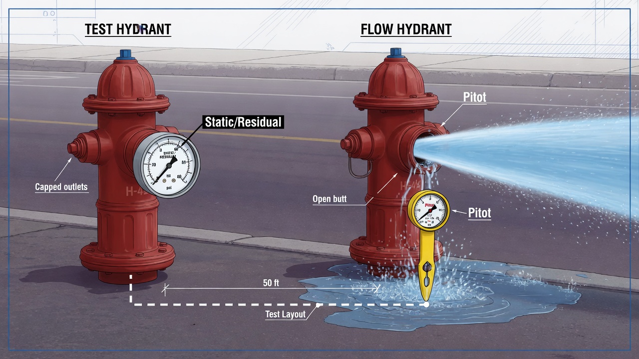
Those inputs begin in the field with three pressure readings and a short list of physical details about the hydrant and its outlets. Capture them cleanly and the math that follows is reliable; blur them and even careful arithmetic will misstate what the system can actually deliver.
Flow tests exist so water-supply evaluation, sprinkler and standpipe design, and hydrant marking rest on measured capacity rather than assumptions. Designers use the results to size fire protection systems against the real main. Fire officials and the AHJ use them to confirm that available flow meets required fire flow. Marking programs use them so a hydrant’s color or tag reflects what it can produce under test, not what a map suggests it should.
Static, residual, and pitot pressure
Every useful test turns on three distinct pressures. Static pressure is the system pressure with no hydrants flowing—the baseline taken at the residual hydrant before any outlet is opened. Residual pressure is the pressure still present at that same hydrant while water is discharging from the flow outlets. Pitot pressure is the velocity pressure read in the center of the discharge stream with a pitot tube and gauge; it is the value that converts into flow rate once the outlet coefficient is applied. Mixing these up—or reading residual on a flowing barrel without a clear residual hydrant—is the most common way a test loses credibility.
Single-hydrant versus multi-hydrant setups
In a single-hydrant setup, one barrel does both jobs: static and residual are read on a gauge port or capped outlet while another outlet on the same hydrant is flowed, and the pitot is taken in that flowing stream. In a multi-hydrant setup the roles split. A residual hydrant carries the static and residual gauges and does not discharge; one or more nearby flow hydrants open while pitot readings are taken at their outlets. Multi-hydrant tests are preferred when higher total flow is needed or when you want a residual reading less disturbed by turbulence at the flowing barrel. In either case, know which gauge belongs where before the first outlet opens.
Field data you must record
Before any calculation, the field sheet should lock down:
- Outlet diameter for each opening flowed
- Outlet type and condition—smooth, rounded, or projecting nozzle; interior condition drives the discharge coefficient
- Number of outlets flowed
- Static, residual, and pitot gauge readings
- Elevation notes between residual and flow hydrants when they sit at different grades
- Hydrant and main identifiers for the report
Those values feed the Q formula that turns pitot pressure into flow in gallons per minute, and from there into the available fire flow projection at a chosen residual used for rating. The next section walks through that formula and the coefficient choices that keep the result trustworthy.
The Q Formula: Turning Pitot Pressure into Flow
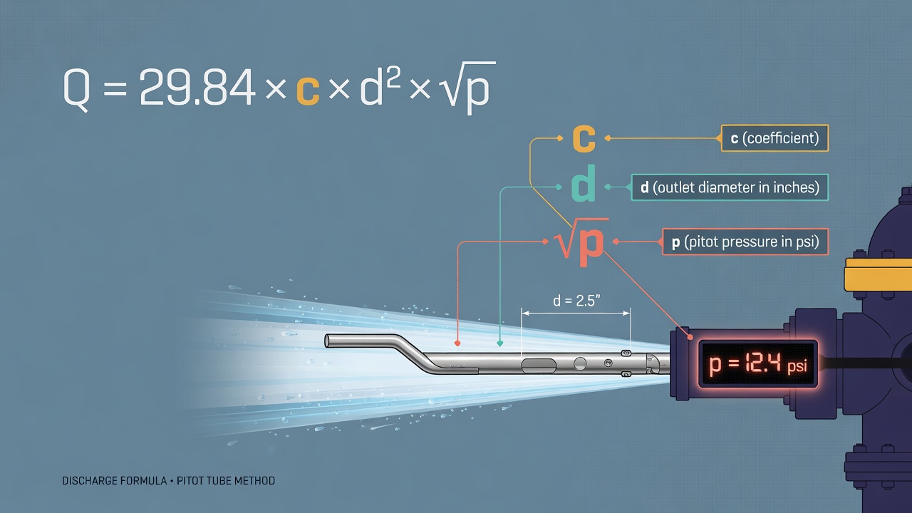
Once you have static, residual, and pitot pressures in hand—and you know which outlets were opened and what condition they were in—the next move is pure calculation. The hydrant flow test formula, often called the Q formula or the pitot gauge flow calculation, converts each pitot reading into a flow rate in gallons per minute. That single equation is the bridge between field gauges and the available fire flow number designers and fire officials will actually use.
In US customary units the standard expression takes this form:
Q ∝ c × d² × √p (scaled by a unit constant into gpm)
Here Q is the discharge from that outlet in gallons per minute. c is the coefficient of discharge (a dimensionless factor that accounts for how smoothly water leaves the orifice). d is the internal diameter of the outlet orifice in inches. p is the pitot pressure in psi, measured in the center of the stream. A fixed unit constant folds together the conversion from theoretical velocity head into gpm when diameter is in inches and pressure is in psi; change the unit system and that constant changes with it.
Why diameter is squared and pressure sits under a square root
Flow is the product of velocity and cross-sectional area. Area of a circular orifice scales with the square of diameter, so d appears as d². Velocity, from Bernoulli, scales with the square root of the velocity head—which is exactly what a properly placed pitot tube reports as pressure. That is why p sits under a radical: double the pitot reading and you do not double the flow; you multiply it by √2, roughly 1.41. Miss either relationship and the result drifts quickly from reality.
Multiple outlets and effective diameter
When two or more outlets are flowed at once, calculate Q for each outlet separately with its own pitot reading, coefficient, and diameter, then add the individual flows. Do not average pitot pressures or plug a single combined diameter into the formula. If a smooth nozzle tip or reducer is attached, the effective d is the internal diameter at the tip’s discharge plane, not the hydrant’s nominal outlet size. Using the wrong d is one of the most common sources of error in a pitot gauge flow calculation.
Unit discipline matters just as much. The customary form expects inches and psi. Metric work (millimetres and kilopascals, or metres and bars) needs its own constant and consistent inputs; mixing systems silently produces nonsense. Keep every length in the same unit family, confirm the pitot gauge is zeroed and reading in the expected scale, and record which coefficient you applied so the next person can reproduce the hydrant flow test formula result without guesswork.
With Q established for the test condition, the same data set is ready for the next step: projecting that measured flow to the available fire flow at a chosen residual pressure. Before that projection, though, the coefficient c deserves a closer look—because a small change in c moves Q as directly as a change in diameter.
Coefficient of Discharge: Matching c to Real Outlet Geometry
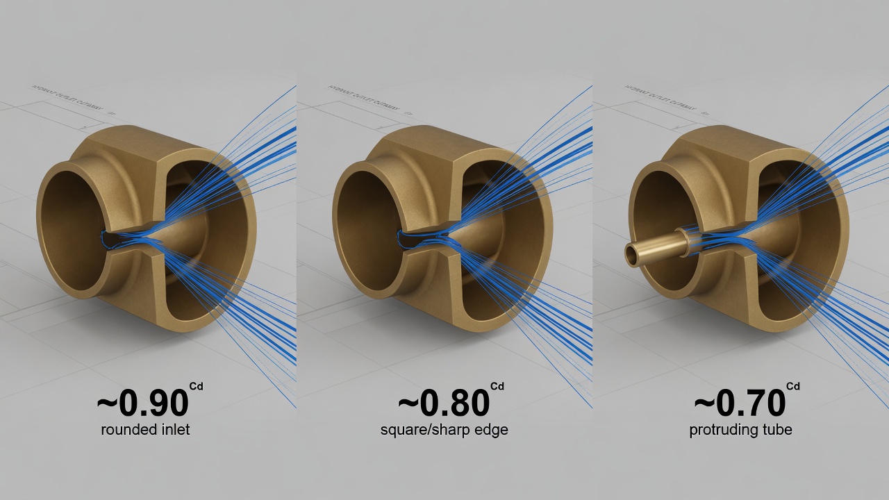
That linear relationship is exactly why the coefficient of discharge cannot be treated as a default or an afterthought. In the Q formula, c is the single factor that corrects pure theoretical orifice flow for the real geometry and edge condition of the hydrant outlet. A frictionless, perfectly formed orifice would use a coefficient of one; every practical outlet falls short of that ideal, so c drops below one in proportion to how the water contracts and loses energy as it leaves the barrel.
Field practice therefore groups outlets by the shape that most influences that contraction. Smooth, well-rounded outlets take a relatively high coefficient. Square and sharp outlets are assigned a lower value. Outlets that form a protruding or projecting tube are given a still lower coefficient. These are starting ranges, not rigid standards. Corrosion, nicks, a partially open gate, or heavy mineral deposits can push the effective coefficient lower than the original casting shape would suggest, so the value must be chosen from what is actually present on the day of the test.
Because Q scales directly with c, an incorrect choice skews every gallon-per-minute figure by the same percentage. Selecting a smooth-outlet coefficient when the true value is closer to a square-outlet figure overstates measured flow by a meaningful fraction; that error then travels straight into the available-fire-flow projection at the chosen residual pressure and gives designers and fire officials an inflated picture of system capacity. The reverse error understates capacity and can force unnecessary upgrades.
For that reason, document the outlet condition thoroughly. Clear photographs of the interior lip, brief notes on rounding or sharpness, and any observed damage or deposits give the authority having jurisdiction a transparent basis for accepting—or questioning—the coefficient applied. Pocket charts that list typical hydrant outlet coefficients are useful field references, yet they remain only a starting point; they never replace looking at the actual outlet and exercising judgment on its condition during the test itself.
Once a defensible c is locked in and Q has been calculated for the test condition, the same data set is ready for the projection that converts measured flow into rated available fire flow.
Available Fire Flow: Projecting Test Results to a Rated Residual
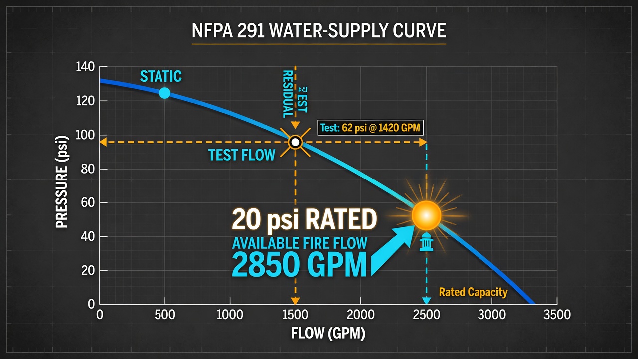
That projection is available fire flow—the predicted discharge the water system can sustain while residual pressure is held at a chosen minimum used for rating. The test flow you already calculated from pitot pressure and the outlet coefficient is only a snapshot at whatever residual the flowing hydrants produced in the field. Designers and fire officials need a standardized rating, so the measured results are scaled along the system’s pressure–flow curve to that common residual benchmark.
The pressure–flow relationship
The widely used form follows a hydraulic relationship common in hydrant-test practice. With QF as the total measured test flow, S the static pressure, F the residual pressure observed while flowing, and R the rated residual you want, available fire flow is:
QR = QF × [(S − R) / (S − F)] raised to a fractional exponent near one-half
That fractional exponent approximates how friction loss and system response change with flow in typical municipal networks. Conceptually, the drop from static to the test residual tells you how far pressure fell for the flow you took; the same ratio, raised to the exponent, estimates how much additional (or less) flow the system can give before pressure reaches the rated residual. If the test residual already sits near the rated target, the factor is close to 1 and QR stays near QF. If the test residual stayed high, the factor grows and the projected available flow is larger than what you measured—provided the system can actually deliver it.
Where the projection stays trustworthy
The math is only as good as the conditions behind the numbers. Keep the rated residual inside a realistic band—projecting far below the pressures you actually observed, or into a range where pumps or PRVs change behavior, stretches the curve beyond what the exponent can represent. Static and residual gauges must be accurate and properly zeroed; a few psi of gauge error moves both the ratio and the final QR. The test should also reflect ordinary system conditions: valves open as they normally are, no temporary boosters, and enough flow that the residual drop is clear and measurable. When those limits are respected, the result is a defensible available-fire-flow figure rather than an optimistic extrapolation.
How the number gets used
Once you have QR at the chosen residual, it feeds the decisions the test was run for. Fire-flow adequacy checks compare that capacity against needed fire flow for the hazard or occupancy. Sprinkler and standpipe discussions use it to confirm that the public supply can support design demand without dropping below minimum residual. Where local practice color-codes hydrants by flow class, the rated available fire flow is the value that places the hydrant in its marking band. In every case the chain is the same: solid pitot work and a correct coefficient produce QF; the pressure–flow projection converts that snapshot into a rated available fire flow others can rely on.
Worked Examples: From Pitot Readings to Rated Available Fire Flow

That same chain is easiest to trust when you can watch the numbers move from gauge reading to rated flow on paper. The examples below use realistic field values, keep every intermediate root and exponent visible, and follow the identical sequence you would use on a clip-board or in a report: choose c, compute each outlet’s Q, sum for total test flow QF, then project to the rated residual with the pressure–flow formula.
Single-outlet Q from pitot pressure
Start with one hose-outlet opening in good condition with a smooth, rounded entrance, so you select a relatively high discharge coefficient. Read a steady pitot pressure in the center of the stream. Square the internal diameter, take the square root of pitot pressure, and multiply through the Q relationship with the unit constant and your chosen c:
Work left to right: apply the unit constant and coefficient first, then scale by diameter squared, then by the square root of pitot pressure. The product is that outlet’s discharge in gpm.
For a quick field note you might round lightly; for a formal calculation sheet keep more precision or round only at the end per local convention. Either way, the arithmetic should stay fully traceable.
Two-outlet test and total QF
Now open a second identical outlet on the same hydrant (or on the flow hydrant in a two-hydrant setup). Take its own pitot reading. Re-use the same coefficient and diameter only if the outlet truly matches; otherwise assign each opening its own values:
Convert the second pitot reading the same way—coefficient, diameter squared, and square root of pressure—to obtain that outlet’s gpm.
Total test flow is simply the sum of the individual outlet discharges. If a third outlet or a pumper nozzle had been flowed, you would calculate its Q the same way and add it. Never average pitot pressures; always convert each reading to flow first, then add.
Projecting to available fire flow at 20 psi
During the test you also recorded static pressure (no flow) and the residual pressure at the gauge hydrant while flowing. Choose the rated residual your report will use. Substitute into the projection formula:
QR = QF × [(S − R) / (S − F)] raised to the fractional exponent
Build the pressure ratio from static, rated residual, and test residual, raise it to the exponent, and multiply by total test flow.
In a formal report most engineers round only at the end according to local convention; on the street a crew might state a lightly rounded available flow at the rated residual. The important point is that every step—coefficient choice, individual Q, summation, pressure ratio, and the fractional exponent—is documented and repeatable.
Work the sequence the same way every time: record outlet diameter and condition → select c → convert each pitot reading to gpm → sum for QF → insert static, residual, and the chosen rated residual into the projection formula → round only at the end according to the audience. Once that habit is automatic, a calculator becomes a speed tool rather than a black box.
Using a Calculator in the Field—Without Treating It as a Black Box

That same sequence is exactly what a good hydrant flow test calculator walks through. You enter each outlet’s diameter and coefficient of discharge, the pitot reading for every open nozzle, the number of outlets flowed, then static and residual pressures plus the rated residual you want. The tool applies the Q formula per outlet, sums to QF, and runs the available-fire-flow projection—returning the same numbers you would get by hand, only faster.
A calculator earns its keep on multi-outlet tests and whenever you need the rated available fire flow on the spot for an engineer or inspector. It also cuts transcription errors when you are juggling several pitot values under time pressure. Hand calculation still matters for training new crew members, for spot-checking a result that looks off, and for understanding why a change in c or residual moves the answer the way it does. Use the tool for speed; keep the method for judgment.
Quick sanity checks before you trust the output
- Residual must sit below static; if it does not, a gauge is wrong or the wrong hydrant was read.
- Pitot pressure should be plausible for the outlet size and how hard the system is flowing—extreme highs or near-zero readings deserve a second look at the tip and the gauge.
- Available fire flow should not leap far above test flow unless there is clear pressure headroom between residual and the rated residual; a huge jump with almost no drop is a red flag for bad inputs.
Document what the calculator used: outlet diameters and condition notes (or photos), the c values you chose and why, every pitot and system pressure, elevation differences if they matter, and the final QF and available fire flow. Engineers, utilities, and inspectors all need that trail so the result can be defended later. Once you know the method, Flows Test is a natural place to run the same math quickly in the field—enter the readings, confirm the sanity checks, and walk away with numbers you can stand behind.