How to Calculate and Apply Friction Loss in Fire Hydrant Flow Tests and Water Supply Evaluations (NFPA 291)

Why Residual at the Hydrant Is Not Supply at the Design Point

An NFPA 291 residual is never a free-floating system pressure. It is the pressure measured at one specific residual hydrant while other hydrants discharge a known flow. That reading belongs only to that hydrant’s location under that flowing condition. The moment your design or evaluation point sits anywhere else on the network—a proposed sprinkler riser, a standpipe inlet, a remote yard hydrant, or a future connection—the residual no longer equals the pressure available there.

Treat the test-sheet residual as if it already applies at the evaluation node and you introduce a systematic error. When the path between residual hydrant and design point runs through smaller mains, longer runs, or extra fittings and valves, friction continues to drop the head. The true residual at the node is lower than the hydrant reading, so the uncorrected value overstates available supply. The opposite can occur when the design node sits on a stronger main path with less intervening loss, or in a more favorable hydraulic position relative to the source; in those cases the raw residual understates what is actually available. Either way, the number on the test sheet is not the number you need.

Friction-loss path accounting is the step that closes that gap. It is the missing link between raw field sheets and usable water-supply input for design or evaluation. It is distinct from C-factor selection, from pitot technique at the flowing outlets, and from how you later graph available fire flow. Those practices matter, but none of them relocate a hydrant residual to a different node. Only identifying the actual hydraulic path and subtracting the losses along it converts the test residual into a defensible pressure at the location that matters.

Mapping the Hydraulic Path: Where Friction Accumulates from Test to Design Point

Ask AI

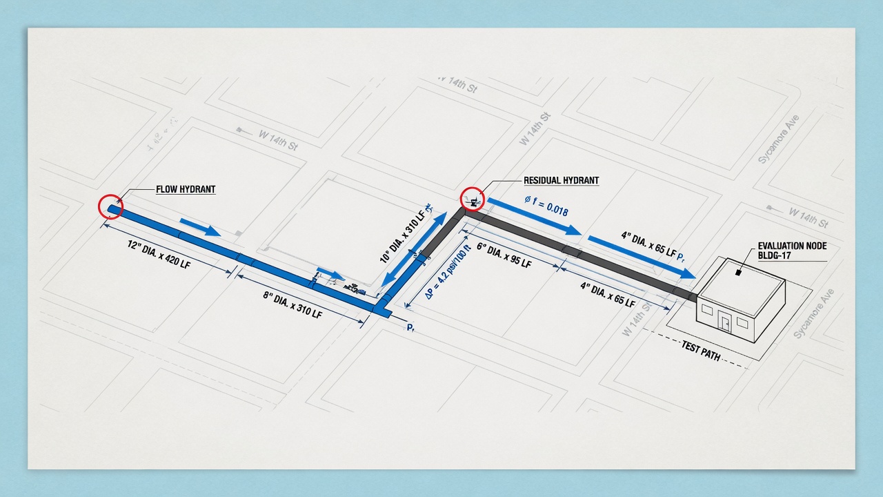
That path is concrete, not theoretical. Sketch it in two legs. The first leg runs from the flowing outlet(s) back through the hydrant barrel and lateral, into the street main, and along the main network to the residual hydrant’s own branch and barrel—the route the test water actually travels while the residual gauge is being read. The second leg is separate: it runs from the residual hydrant’s location (or the nearest main node) along the mains, services, and private fire piping that reach the building connection, sprinkler tap, or rating point you care about. Drawing both legs keeps the test hydraulics distinct from the evaluation hydraulics so you never double-count or omit a segment.

What the residual already includes—and what it does not

Friction that occurs on the first leg while the test is flowing is already embedded in the residual reading. Losses through the flowing hydrant’s outlet, any test hose or playpipe, the street mains carrying that flow, and the residual hydrant’s lateral and barrel have already lowered the pressure at the gauge. You do not subtract those again when you move the result to another node. What you do apply after the test are the losses (or gains) on the second leg—the path that carries the design or evaluation flow from the residual location to the point of use. Only the segments that actually convey the relevant flow rate at the condition you are evaluating belong in that correction. Idle branches, closed laterals, and parallel mains that carry none of the design flow contribute nothing and stay out of the arithmetic.

Segments that usually dominate the correction

A few components repeatedly produce the largest pressure drops between residual hydrant and design point. Undersized hydrant laterals—short runs of small-diameter pipe between the main and the hydrant shoe—can drop several pounds even at moderate flows and affect both the residual itself and any nearby evaluation node. Long dead-end mains concentrate the entire test or design flow into a single path with no intermediate reinforcement, so length and diameter matter heavily. Small-diameter service lines or private fire mains that leave the public main and run to the building or yard hydrant are equally common culprits; their length, fittings, and any meter or backflow assembly sit squarely on the second leg and must be accounted for at the design flow. Once those high-impact segments are identified and the idle ones discarded, the path is ready for the segment-by-segment formulas that convert length, diameter, and flow into friction loss.

Turning the Path into Numbers: Hazen–Williams, Outlets, and C-Factors

The segment calculation turns each run into a pressure drop. With the second-leg path defined, every main segment is evaluated with the Hazen–Williams friction-loss relationship used throughout fire-protection supply work. In the form that returns loss directly in psi, the expression is:

ΔP = 4.52 × L × Q^1.85 / (C^1.85 × d^4.87)

Here Q is the flow carried by that segment (gpm) under the evaluation condition—not necessarily the test flow if the design demand differs—C is the Hazen–Williams roughness coefficient, d is internal diameter in inches, and L is length in feet. Because the exponents are steep, small errors in diameter or C move the result more than modest errors in length. Apply the formula once per continuous run of uniform pipe; change diameter, material, or age class and you start a new segment. Fittings and valves on that run are usually converted to equivalent length and added to L, or treated as separate concentrated losses if their K-values are known.

Concentrated losses at outlets, gates, and test hose

Pipe friction is only part of the path. Concentrated losses appear wherever the water changes direction or velocity abruptly. On the flowing hydrant, outlet geometry, the open steamer or hose gate, and any length of test hose or diffuser between the butt and the pitot tip all drop pressure before the residual gauge ever sees the main. Those first-leg losses are already embedded in the residual reading you recorded, so you do not subtract them again when correcting to a remote node. What you do account for on the second leg are gates, meters, backflow preventers, and hydrant laterals that lie between the residual hydrant and the design point and that will carry evaluation flow. Manufacturer head-loss curves or published equivalent lengths for those devices keep the accounting consistent with the pipe segments.

Choosing C for supply evaluation

C is not a nozzle discharge coefficient; it describes interior roughness of the conveyance pipe. For supply evaluations, select C by material and expected condition rather than by optimistic catalog values. Cement-lined ductile or cast iron in good service typically supports a higher C than unlined or tuberculated older iron. PVC and other smooth plastics sit at the high end when joints are clean. Age, tuberculation, and soft-water or aggressive soils push C downward—sometimes sharply on unlined mains—so a conservative mid-life value is safer than a new-pipe assumption when the evaluation is for fire flow or sprinkler demand. When segments of different materials sit on the same path, assign each its own C; do not average them into a single fictitious coefficient.

Units and direction of the sum

Keep every input in the unit set the formula expects: flow in gpm, diameter in inches, length in feet, result in psi. Mixing feet of head with psi, or nominal diameter with actual internal diameter, is the most common arithmetic failure in path corrections. Once each segment and each concentrated device has a ΔP at the evaluation flow, add those losses in the direction water will travel from the residual hydrant toward the design or rating node. The residual pressure minus that total path loss is the pressure available at the node under the test’s flowing condition—ready for the worked correction that follows.

Worked Correction: From Residual Hydrant to Pressure at the Design Node

Ask AI

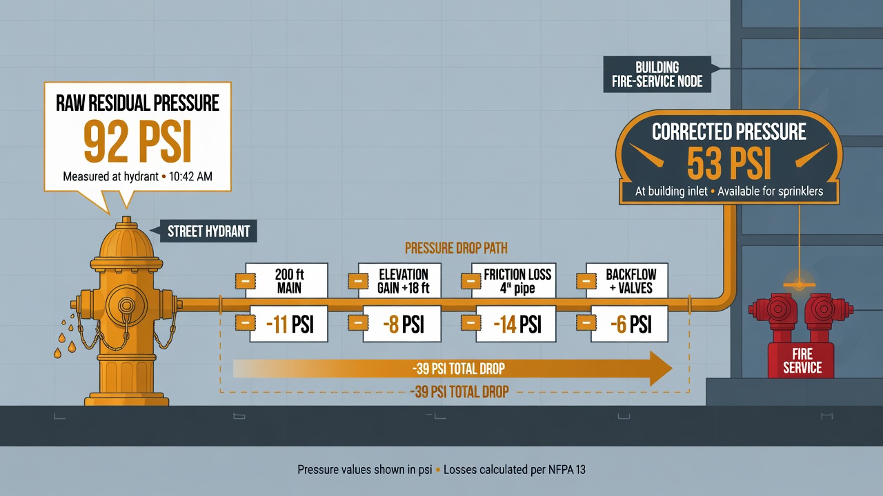
That residual-minus-total-path-loss figure is exactly the pressure that belongs at the evaluation node under the same flowing condition the test just produced. A short numeric walk-through makes the arithmetic and the sign convention concrete.

Weaker remote node: subtract the second-leg loss

Consider residual hydrant R reporting 48 psi residual while the test flows 1,200 gpm. The second-leg path from R to building node B consists of 320 ft of 8-inch ductile-iron main (C = 120) followed by 80 ft of 6-inch private lateral (C = 100) and one fully open 6-inch gate valve. At the 1,200 gpm evaluation flow, Hazen–Williams yields roughly 3.8 psi on the 8-inch segment and 9.1 psi on the 6-inch lateral; the gate adds another 0.6 psi of concentrated loss. Summed path loss is therefore 13.5 psi.

Because node B lies downstream of R on this flow pattern—water must travel farther from the strong supply to reach B—the node is hydraulically weaker. The correction is subtraction:

P at B ≈ 48 psi − 13.5 psi = 34.5 psi

under the identical 1,200 gpm system demand. That 34.5 psi is the residual pressure that actually exists at B while the test outlets are still flowing; it is the value you carry forward into any later available-fire-flow calculation for the building.

The correction form and the sign convention

The general form is simply:

P_node ≈ P_residual hydrant ± ΣΔP (segments + devices)

Use the minus sign when the node is on the weaker side of the residual hydrant (farther from supply or on a smaller main). Use the plus sign when the node sits on a stronger path.

Stronger upstream tap: add the intervening loss

A second, briefer case shows why the sign matters. Suppose the same test still shows 48 psi at R, but building node B taps a large feeder main only 40 ft from a strong grid intersection, while residual hydrant R is 500 ft out on a 6-inch dead-end spur. During the test, flow is traveling past B toward R. Friction between B and R is 7 psi at test flow. Blindly adopting the 48 psi residual would understate supply at B; the correct move is addition:

P at B ≈ 48 psi + 7 psi = 55 psi

at the same flowing condition. Using the raw residual here would have been conservative, yet for the wrong hydraulic reason—and would have hidden how much stronger the true tap really is.

In both cases the corrected pressure remains tied to the test’s flowing rate and residual condition. No elevation adjustment and no projection to a different flow have been introduced yet; those steps come only after the friction path has been closed.

Elevation Head Comes Next—and Must Stay Separate from Friction

With the friction path closed at the test’s flowing residual, the next correction is elevation head. Elevation is a static geometric shift: it depends only on the vertical distance between the residual hydrant and the design or evaluation node, not on how much water is moving. Friction, by contrast, scales with flow. Mixing the two—or applying either more than once—produces a pressure that no longer represents true available supply at the node.

The clean sequence is straightforward. Start from the residual pressure already adjusted for second-leg friction under the test flowing condition. Then move that pressure from residual-hydrant grade to design-node grade with a pure elevation correction. Only after both steps does the result sit at the right location and the right elevation for the rate that was flowing during the test. If a later fire-flow projection or a different evaluation rate is needed, friction is recalculated for that new rate; elevation is left unchanged because the geometry has not moved.

Failure modes that quietly ruin the result

Two errors appear repeatedly on hilly sites and on tall private risers. The first is counting elevation twice—once inside an informal “equivalent length” or adjusted C-factor and again as an explicit head term. The second is folding elevation into the friction calculation itself so that a flow-dependent formula is forced to carry a static offset. Either mistake overstates pressure when the node is downhill from the residual hydrant and understates it when the node is uphill. Private mains that climb several stories inside a building are especially unforgiving; a single double-counted rise can erase the margin the system actually has.

Keep the datum consistent from test to evaluation. NFPA 291 flow-test records normally note residual-hydrant elevation or a local benchmark. Use that same reference when you establish design-node grade. Switching datums mid-calculation reintroduces the very offset you are trying to remove and leaves the corrected pressure floating relative to the rest of the supply analysis. Once elevation and friction are each applied once, in the proper order, and against a single vertical reference, the path-corrected pressure is ready for fire-flow rating and supply evaluation work.

Feeding Path-Corrected Pressures into Fire-Flow Ratings and Supply Evaluations

With friction and elevation each applied once against a single datum, the path-corrected residual—and its companion static, adjusted the same way—become the pair you feed into every supply calculation at the node of interest. When you project available fire flow or build a supply curve there, those corrected values replace the raw hydrant residual and static as the starting points. The graphing and rating methods themselves do not change; only the input pressures move so they represent the true hydraulic location rather than the test hydrant. Using the uncorrected hydrant pair would simply re-import the path error the preceding steps removed.

The same corrected pair anchors sprinkler water-supply evaluations and municipal supply write-ups whenever the connection point differs from the residual hydrant used in the NFPA 291 test. That connection may be a riser base, a private fire-service main tap, a yard hydrant, or a rating node several blocks away. Document residual and static at the actual point of connection so the hydraulic calculations that follow—demand checks, duration estimates, or system curves—start from pressure that already accounts for intervening mains, fittings, and grade.

What to Record with Every Correction

A defensible correction leaves a clear audit trail. Capture at least the following so a reviewer can reconstruct the path and the arithmetic:

• Path sketch showing the residual hydrant, the design or evaluation node, and every main segment between them
• Diameter, length, and C-factor assigned to each segment
• Flow rate used for each friction-loss calculation along that path
• Elevation datum and the grade difference applied between hydrant and node
• Final corrected residual and static pressures at the node under the test flowing condition

When a Single Distant Residual Is Not Enough

Path uncertainty grows with distance, undocumented private mains, unknown fittings, or long dead-ends whose actual C-factors cannot be confirmed. When the correction itself would rest on too many assumptions, stretch a second residual location closer to the node—or run a main-capacity style setup that measures residual nearer the evaluation point. Those field choices keep the friction accounting short enough to stay credible rather than forcing a single distant residual across an opaque network. Once the corrected pair is in hand and the supporting notes are complete, the numbers are ready for the field checks that confirm the assumptions still hold.

Field Checks That Keep Friction Assumptions Defensible

Those checks start with the map itself. Before diameters and C-factors are locked into the Hazen–Williams segments, cross-check GIS or main maps against valve cards, as-built sketches, and any known rehab or lining history. A main that still appears as unlined cast iron on the system diagram may already have been cement-lined or replaced; treating it as the older material understates available pressure at the node. The reverse error—assuming a smooth modern C on pipe that was never upgraded—overstates supply. Resolve those conflicts on paper before the correction is treated as final.

Pay special attention to everything between the public residual hydrant and the building or design node. Private fire mains, detector-check or compound meters, backflow preventers, and undocumented reducers frequently dominate second-leg loss even when the public main looks generous. If the path sketch cannot confirm size, length, and fitting inventory on the private side, treat those segments as high-impact unknowns rather than guessing a diameter that makes the arithmetic tidy.

When to stop correcting and retest instead

Use a simple decision rule: if the cumulative uncertainty in length, diameter, or C rivals the magnitude of the friction correction you are about to apply, do not force a paper adjustment from a distant residual. Move the residual hydrant closer to the node, or add a second test that shortens the unknown path, and rebuild the corrected pair from the tighter geometry. Over-correcting on thin data produces a number that looks precise and travels into ratings and evaluations with false confidence.

Friction-specific mistakes to catch before sign-off

A short list of path errors still appears often enough to warrant a final pass:

• Using the wrong flow in Hazen–Williams—total test flow when only the share that actually travels the second-leg segment belongs in Q
• Ignoring laterals or private stubs that carry design flow even though they never appeared on the original hydrant-to-hydrant sketch
• Mixing first-leg test-hose or outlet loss into the main-path correction after the residual has already absorbed those losses

Catch those three and the path-corrected residual remains tied to the physical network rather than to an optimistic spreadsheet. With the field checks closed, the NFPA 291 residual has been converted into a defensible supply figure at the node that matters—ready for fire-flow projection, sprinkler evaluation, or the municipal record without pretending the hydrant and the design point are the same place.