
How to Graph and Interpret Fire Hydrant Flow Test Results: Residual Pressure Curves, Available Fire Flow & NFF Calculations (NFPA 291)
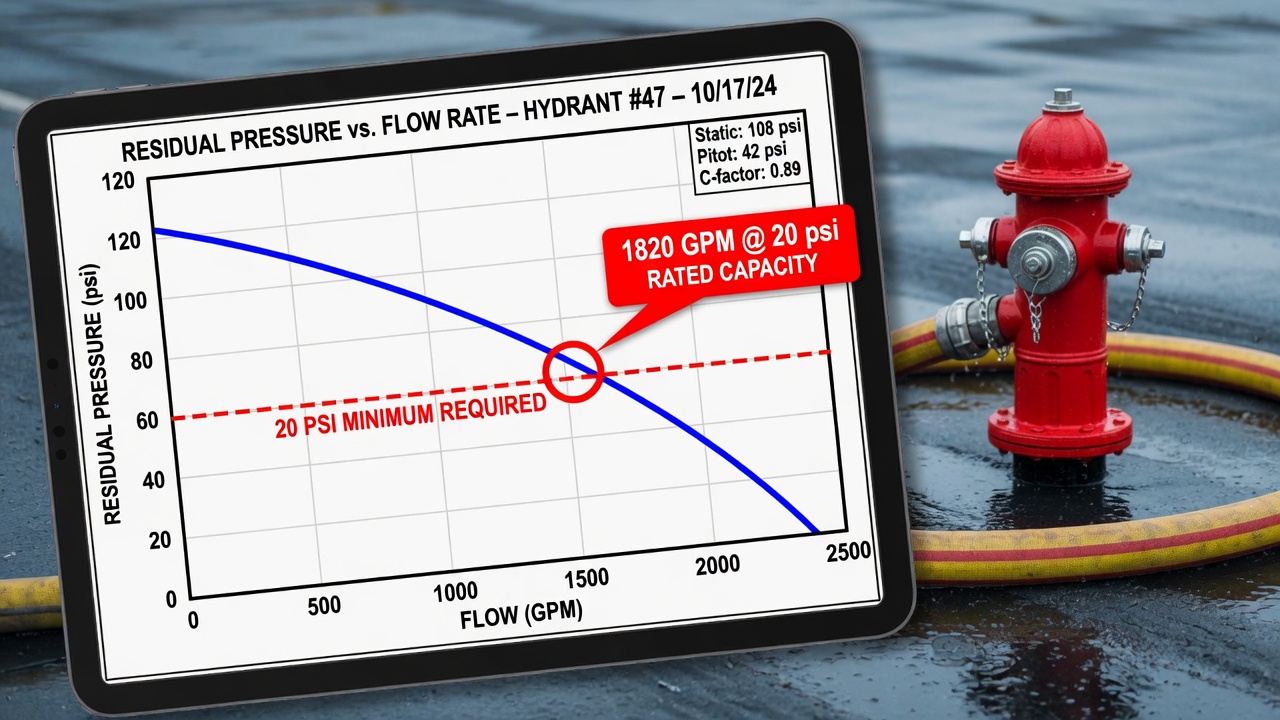
A fire hydrant flow test is only half done when the gauges come off the steamer. Static pressure, residual pressure, and pitot readings become useful when you turn them into a residual pressure curve—the graph that shows how system pressure falls as you pull more flow. From that curve you can read available fire flow at 20 psi, estimate hydrant or system capacity, and support NFF (needed fire flow) and water-supply evaluations without treating the NFPA 291 formulas as a black box.
This article walks through that process end to end: converting pitot readings to GPM, plotting static and residual points on the right scale, drawing the residual-pressure curve, and reading 20 psi available fire flow and rated capacity from the finished chart. You will also see how multiple flowing hydrants, elevation, and friction losses affect the plot, which graphing mistakes skew the answer, and when a spreadsheet or software tool is worth using instead of paper. The goal is a clear, defensible residual-pressure curve you can hand to a designer, AHJ, or insurer with confidence.
Why the Residual-Pressure Curve Beats Formula-Only Fire Flow Math
That confidence rests on treating the residual-pressure curve as the primary rating deliverable—not a decorative chart you draw after the formulas are finished. Under NFPA 291 practice, the graph of residual pressure against flow is how available fire flow at 20 psi and system capacity get communicated. The plot is the answer; the equations are only tools that help you build it.
When several flow points—or intermediate residuals from more than one flowing hydrant—are available, the slope of the line shows how strong the main really is. A steep drop means the network loses pressure quickly under demand; a flatter slope means it holds better as outlets open. Point scatter is just as revealing: tight clustering builds confidence that the 20 psi intercept is trustworthy, while wide scatter flags a weak test, a gauge problem, or an unaccounted elevation or friction effect that should be resolved before any number is reported.
A one-shot available-fire-flow formula can produce a single GPM from static pressure and one residual, but it hides the shape of the supply. Plot the curve and you see whether the system behaves as expected on the scale NFPA 291 uses, whether an intermediate point sits off the line, and how far you can safely extrapolate. That visual check is what turns raw field readings into a defensible rating a designer, AHJ, or insurer can actually use.
Scope here stays at the desk. Field hookup, pitot technique, and gauge placement belong in separate procedure material. The work in the sections that follow is converting those readings into plottable points, drawing the residual-pressure curve, and reading available fire flow and NFF capacity straight from the graph.
From Gauge Readings to Graph-Ready (Q, P) Points
That conversion starts by turning every field reading into a clean coordinate the residual-pressure curve can actually use. Each plotted point is a paired (flow in GPM, residual pressure in psi) value. Flow sits on the horizontal axis; residual pressure sits on the vertical. The static reading belongs on the same pair of axes at zero flow—the left-hand intercept that anchors the entire curve before any water is discharged.
Getting the flow half of each coordinate is a short, purpose-built step—not a full hydraulic calculator tutorial. From the pitot (velocity-pressure) reading at an open outlet, apply the standard discharge relationship that multiplies the outlet’s coefficient and cross-section by the square root of the pitot pressure. The result is discharge in GPM for that outlet alone. You only need enough accuracy to place the point on the graph; the curve, not the intermediate arithmetic, is what NFPA 291 uses for available fire flow and NFF.
Single-outlet versus combined multi-hydrant totals
When only one outlet is open, that single calculated GPM is the x-coordinate paired with the residual pressure observed at the same moment. When two or more outlets—or entire hydrants—flow together, add every individual discharge so the residual pressure recorded during the simultaneous flow is plotted against the combined total Q. Mixing a partial total with a system-wide residual is one of the fastest ways to warp the slope and misread the 20 psi intercept later.
Minimum data package before any axis is drawn
Do not sketch scales until every item below is in hand. Missing any one of them leaves a gap you cannot honestly fill on the plot:
- Static pressure (no-flow condition)
- Residual pressure at each distinct flow condition
- Pitot (velocity) pressure for every flowing outlet
- Outlet diameters (or nozzle sizes)
- Outlet coefficients or nozzle factors used in the discharge conversion
With that package complete, every (Q, P) point—and the static intercept at Q = 0—is ready for the axes. The next move is choosing scales and locking in the 20 psi reference line so the residual-pressure curve can be drawn and read directly.
Lay Out the Axes, Choose Scales, and Draw the 20 psi Line
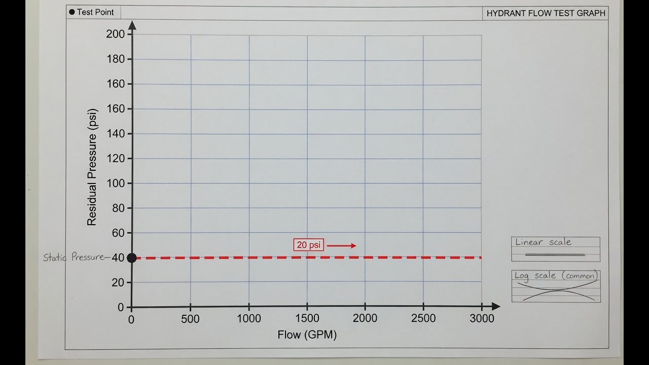
Choosing scales starts with locking the axis orientation that residual-pressure curves expect. Discharge—total flow in GPM—runs along the horizontal axis; residual pressure in psi runs vertically. Static pressure is marked on the pressure axis at Q = 0, the left-edge intercept that anchors every curve you will draw.
Paper choice shapes how that curve looks and how easily you read it. On ordinary linear paper both axes are arithmetic, so the residual trend bows: head loss rises roughly with flow to the 1.85 power, and the line from static through your test points curves downward. Semi-log layouts put flow on a logarithmic scale (pressure stays linear). That arrangement straightens the Hazen-Williams relationship, so two or more flow points fall closer to a straight line and the 20 psi intercept is easier to fit and read. Log-log paper can do similar work when both axes benefit from compression. Use linear paper when you want the physical shape of the drop visible; use semi-log when clean fitting and extrapolation matter more.
Either way, set the ranges so static, every measured residual, and the 20 psi floor all sit comfortably on the chart. If static is high and your lowest test residual is still well above 20 psi, leave headroom above static and open space below the lowest residual—do not crush the lower end of the pressure axis or the intercept will be hard to judge. On the flow axis, extend past the largest combined discharge you recorded so the eventual available-fire-flow reading is not hanging off the right edge of the sheet.
Place the horizontal 20 psi reference line first—before plotting points or sketching any curve. That line is the rating target: available fire flow is simply the Q value where the residual-pressure curve crosses it. Drawing it at the start turns the intercept into a deliberate read rather than an afterthought once the curve is already inked. With axes, scales, and the 20 psi line locked, the graph is ready for the (Q, P) points and the fit that follows.
Fitting the Residual Curve with the 1.85-Power Relationship
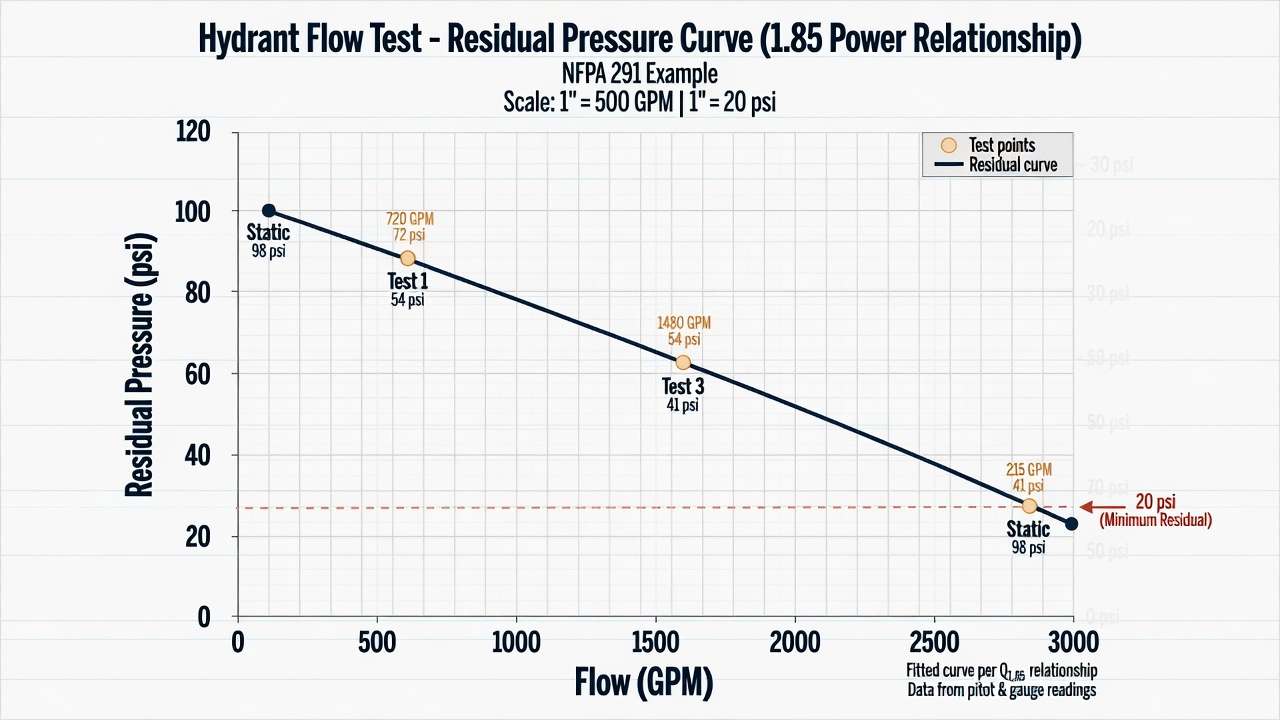
Plot the static pressure first—the anchor at zero flow on the vertical axis. Then place each measured residual at its corresponding total flow on the horizontal axis. Those (Q, P) points are not joined with a freehand sketch; they are governed by the industry relationship that pressure drop from static scales with flow raised to the 1.85 power. Once the points are down, the residual curve is the line (or gentle curve on linear paper) that satisfies that exponent from the static intercept through the data.
Two-point method versus multi-flow tests
A classic two-point fit uses only static pressure and one flowed residual. With those two anchors you can project the 1.85-power line all the way to the 20 psi reference and read available fire flow. The method is fast and fully acceptable when only one hydrant can be flowed, but it hides any measurement scatter. Multi-flow tests—two or more residual points at different total discharges—expose that scatter. Points that sit cleanly on a common 1.85 slope confirm a sound test and a strong main; an outlier flags a sticky gauge, an unrecorded elevation change, or a partial valve opening. In that case you improve the fit by giving honest weight to the consistent points rather than forcing the line through every mark.
Why a log plot straightens the residual line
On ordinary linear paper the residual-pressure trend bows because drop is proportional to Q1.85. Re-plot the same data on semi-log or fully logarithmic axes (or on a transformed spreadsheet chart that graphs pressure drop against Q1.85) and the relationship becomes an approximately straight line. That straightness is what lets you draw or regress the fit with a straightedge or a simple linear trend, then transform back if needed. Do not drag the line through a clearly bad point; note the anomaly, exclude it from the regression, and keep the slope that the reliable observations support.
Hand-drawn NFPA sheets and spreadsheet charts
On traditional NFPA-style graph paper, mark static, drop the residual points in pencil, then lay a straightedge along the log-scaled trend and ink the line lightly so erasures remain possible. Leave a short tick or note beside any discarded outlier. In Excel or Google Sheets, enter static and residual pairs, add a column for Q1.85 or switch the chart axes to logarithmic, and fit a linear trend line through the trustworthy points only. Format the chart so the 20 psi reference already drawn on the sheet remains visible; the fitted line will cross it cleanly and hand the next reader a ready intercept. Either medium—pencil on log paper or a transformed spreadsheet chart—produces the same residual-pressure curve the standard expects, ready for the available-fire-flow reading that follows.
Reading Available Fire Flow at the 20 psi Intercept
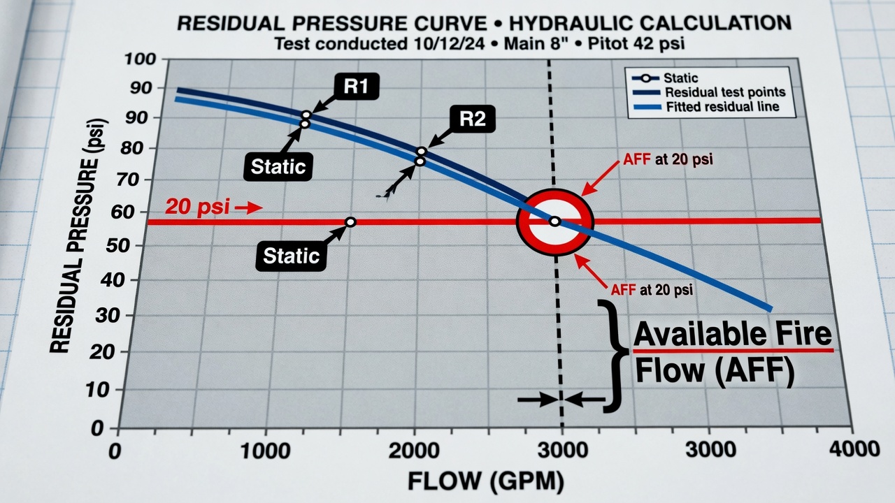
With the residual-pressure curve fitted and the 20 psi reference already on the sheet, available fire flow is simply the discharge at which that curve crosses the line. Drop a vertical from the intersection to the flow axis and read the GPM value—the graph’s primary deliverable under NFPA 291. That single intercept is the system’s rated capacity at the residual pressure commonly accepted as the practical floor for fire-stream effectiveness; everything else on the chart supports or qualifies it.
When a measured residual already sits near or below 20 psi, the intercept is found by interpolation rather than extension. Locate the two plotted points that straddle the reference line (or the single point just above it and the static anchor). On linear paper the eye can split the vertical gap proportionally; on a log or Q1.85 plot the same proportion is taken along the straightened segment. Mark the crossing, drop to the GPM scale, and record the value. Because the data already bracket the target residual, confidence in the reading is high and no additional assumptions are required.
When every residual remains well above 20 psi, controlled extrapolation along the same 1.85-power line is required. Continue the fitted curve downward until it meets the reference line, then read the corresponding flow. Keep the extension short: the farther the intercept lies beyond the highest test flow, the more sensitive the result becomes to small errors in slope or coefficient. If the projected point is more than roughly twice the largest measured Q, treat the number as indicative only and note the limitation on the report. Never force the line through an outlier simply to reach 20 psi sooner.
Finally, state the intercept in plain report language that carries its own context. Write the available fire flow together with the test configuration—which hydrants were flowed, which served as residual gauges, outlet sizes and coefficients used, and whether the residual basis is a single hydrant or a network average. A bare GPM figure stripped of that framing invites misapplication; the graph-plus-sentence package lets the next engineer or AHJ reuse the result without re-deriving the curve.
Reading Rated Capacity and Framing NFF from the Same Curve
Available fire flow is only the first value you take off the residual-pressure curve. With that intercept fixed at 20 psi, the same curve still has more work to do: it also supplies the rated hydrant capacity that many local authorities and ISO practices expect, and it frames the comparison against needed fire flow.
Rated capacity (sometimes called hydrant capacity) is read from the fitted curve at the residual-pressure basis the rating method actually uses—not automatically at 20 psi. When local or ISO practice rates a hydrant at a higher residual (for example the residual observed during the test, or another specified floor), drop a horizontal line at that pressure, find where it meets the curve, and read the corresponding GPM. That value is distinct from available fire flow. Report both when the two bases differ: AFF at 20 psi for system-supply language, and rated capacity at the method’s residual for the hydrant rating itself. Never force the rated-capacity callout onto the 20 psi line just because AFF already lives there.
Needed fire flow (NFF) is not a second intercept you invent on the axes. It is the demand-side target—the flow the occupancy or code calculation requires. You compare the graphical available fire flow against that NFF figure off-chart. If AFF meets or exceeds NFF, the supply side of the check is satisfied; if it falls short, the gap is a supply shortfall, not a drafting error on the residual curve. Keep sprinkler demand calculations and full ISO scoring out of this step; the finished graph simply hands those later evaluations a clear, configuration-tied supply number.
Minimum annotations on a finished graph
Before the sheet leaves the desk, every plot should carry the callouts below so the next reader can reuse the result without reopening the field notes:
| Annotation | What to show |
|---|---|
| Static pressure | Q = 0 intercept, labeled in psi |
| Test points | Each (total Q, residual P) pair plotted and tagged |
| Fitted residual curve | 1.85-power curve through static and valid points |
| 20 psi AFF | Horizontal reference line and GPM intercept callout |
| Rated capacity | Callout at the residual basis used for rating (if different from 20 psi) |
| Test identity | Date, location, flowed hydrant IDs, residual gauge hydrant(s) |
With those marks in place, the graph is no longer a sketch of field data—it is the rating deliverable that carries both supply figures and the context needed to compare them with NFF.
Diagnosing the Residual Curve: Slope, Elevation Offsets, and Extrapolation Traps
That rating deliverable still has to earn its trust. Before anyone treats the 20 psi intercept or rated capacity as final, the shape of the curve itself becomes a quality check—graph-first QA that catches weak mains, setup errors, and plotting mistakes the formulas alone would hide.
What slope is telling you
A steep residual-pressure drop with only modest flow increase is a classic weak-main or bottleneck signature. Friction loss is dominating; a partially closed valve, undersized segment, or long run between the residual hydrant and the flowed outlets will pull the curve down hard. The opposite pattern—an unusually flat slope where residuals barely move while flow climbs—usually points the other way: a stuck or misread gauge, an outlet coefficient that is too optimistic, or a test layout so close to a strong feed that the residual hydrant never feels the draw. Either extreme means the plotted points do not yet describe true main capacity.
Elevation offsets before you trust the line
When residual and flow hydrants sit at different elevations, the pressures you plot must be shifted to a common datum before the curve is fitted. Uncorrected elevation differences tilt the entire residual line and move both the 20 psi intercept and any rated-capacity reading. Correct first, then fit; never treat raw gauge values as interchangeable across a grade change.
Graphing failures that invent capacity
Several desk-side mistakes produce a clean-looking curve that is still wrong. Wrong log cycles squash or stretch the 1.85-power relationship so the “straight” fit is an illusion. Forcing the line through obvious outliers drags the intercept. Extrapolating far beyond the highest measured flow invents capacity the test never proved. Ignoring velocity pressure when the residual reading was taken on a flowing outlet understates true residual and inflates available fire flow. Each of these is visible on the finished graph if you look for them.
Reject-or-retest checklist (curve-driven)
- Slope far steeper or flatter than expected for known main size and length?
- Elevation difference between residual and flow hydrants left uncorrected?
- Fitted line forced through clear outliers instead of reflecting the reliable cluster?
- Extrapolation extending well past the highest measured flow?
- Velocity pressure omitted when residual was taken on a flowing outlet?
- Wrong paper or log cycle so the power relationship does not straighten?
If any answer is yes, reject the graph and retest or replot before the numbers leave the desk. Done right, the residual-pressure curve is both the calculation and the audit trail—supply figures you can defend, and a picture that shows why they hold.